Abstract
Memory traces used in high-performance computing (HPC) studies can reach gigabytes, making them expensive to distribute and replay. This work asks whether a small learned artifact can generate proxy traces that reproduce the cache hit rates of larger source traces. An initial long short-term memory (LSTM) codec encoded fixed windows of signed address deltas. Although it sometimes reached very low reconstruction loss, it did not reliably preserve cache behavior.
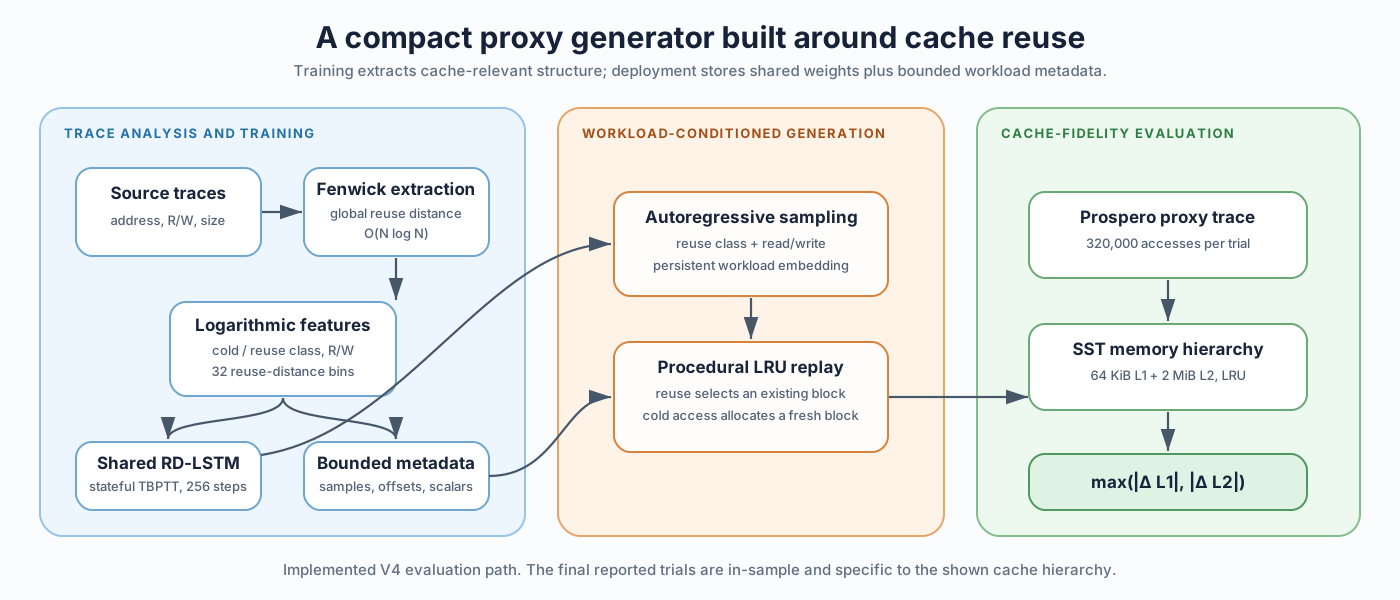
The redesigned generator models logarithmically binned reuse distance instead of address deltas. A Fenwick tree extracts reuse distances in time; a workload-conditioned stateful LSTM predicts reuse classes and read/write operations; and an LRU-stack replay procedure maps predicted reuse positions back to exact previously generated block identities. Trace-length-dependent latent sequences are replaced with bounded workload metadata.
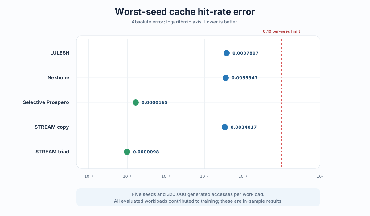
The frozen shared model and metadata for five workloads occupy 565,681 serialized bytes. Across five in-sample trials of 320,000 generated accesses per workload, the largest observed absolute cache hit-rate error was 0.0037807 under the evaluated SST cache configuration.
1. Introduction
The goal of this program is to create a trace codec that fits in L2 cache while preserving cache behavior of HPC traces. Two metrics measured the goal of the project:
- Accuracy between generated and original trace must not differ > 10%
- Model + Deployed Artifacts < 2 MB (L2 cache size)
2. Previous Design Decisions / Alternatives tried
Before settling on the final iteration of the architecture used, a one channel LSTM used to only predict deltas was used. MSE drops in training proved LSTM architecture can learn trace reconstruction, so we added a second channel to also predict read and write flags.
Multiple problems from early iterations of the architecture:
- Subpar accuracy when validating cache behavior: proving a decrease in MSE does not correlate with cache behavior
- Artifact size increasing/ scaling with trace length: Generated Models and latents scaled with size of traces, so a big trace thats is 1.5GB long compresses to 500mb, which doesn't fit in L2 cache
- Models learned did not used a unified model: Each time a new trace is fed through the model, the model needed to be retrained on a different trace, increasing size of artifacts (latents).
Using delta sequence as an indicator for training led to subpar accuracy. This is due to the model learning trace sequences from a specific trace and deltas shifts in traces leading to new reconstructions that impact model performance. Low training loss also does not correlate with cache fidelity enough to produce accurate enough traces. Furthermore, small prediction errors accumulate through the address cumulative sum.
| Model | Reported normalized-delta MSE | SST worst hit-rate error | Outcome |
|---|---|---|---|
| Ordered-latent delta LSTM, | 0.00003 | 0.834683 | Fail |
generated_address[t] = generated_address[t-1] + predicted_delta[t]
Since every new address depends on the previously generated address, we carry the prediction error forward. Tiny address errors impact hit and miss rates.
3. Reuse Distance
The model predicts logarithmic reuse-distance bins as a more accurate metric for cache behavior. This addresses the problem of using delta sequences by reconstructing repeated blocks through predicting LRU-stack positions.
Simple example:
blocks 0,1,2,3

Final block says to reuse the block at stack depth 2
The LRU-stack replay selects the exact earlier block, which removes the need for cumulative address addition. Predicted reuse position leads to exact existing block identity. The new blocks are allocated only for predicted cold accesses, and reuse accesses always return to a block that already exists.
Runtime of Reuse Distance - Fenwick Tree
The concern of using reuse distance is the runtime being O(n^2). By using a fenwick tree, the runtime is reduced to o (n logn). The Fenwick tree computes how many distinct cache blocks have been accessed since that block was last used by keeping a marker of its most recent access position.
Example trace:
pos: 1 2 3 4 5
block: A B C A B
Fenwick tree:
A -> position 1
B -> position 2
C -> position 3
position: 1  2  3
marker:   1  1  1
When a reuse happens at position 4 where block A appears again, A's marker moves. First the prefix is calculated:
prefix(3) - prefix(1)
= 3 - 1
= 2
Those two blocks are B and C, so A’s reuse distance is 2.
The algorithm then moves A’s active marker:
remove marker at position 1
add marker at position 4
Active markers become:
B -> position 2
C -> position 3
A -> position 4
Fenwick Tree operations: Prefix
prefix(i) returns the number of active markers from position 1 through position i:
def prefix(i):
    total = 0
    while i > 0:
        total += tree[i]
        i -= i & -i
    return total
Update
add(i, value) changes the marker at position i:
def add(i, value):
    while i <= n:
        tree[i] += value
        i += i & -i
Complete algorithm
For access position t and block b:
previous = last.get(b)

if previous is None:
    rd[t] = COLD
else:
    rd[t] = prefix(t - 1) - prefix(previous)
    add(previous, -1)

add(t, +1)
last[b] = t
The tree contains only the latest occurrence of each block. Therefore, counting active markers between two positions counts distinct blocks instead of total accesses.
Time and Space Complexity
Each prefix query or update touches at most O(log N) tree entries.
Per cold access:
1 update
Per reused access:
2 prefix queries
2 updates
Overall:
Time:   O(N log N)
Memory: O(N + U)
Where N is the number of accesses, and U is the number of unique blocks.
4. Classification
Reuse distance spans cold accesses, immediate reuse, and reuse separated by millions of distinct blocks. Direct regression over that range gives large distances disproportionate influence and makes cache-capacity boundaries difficult to learn.
The representation uses:
bin 0 = cold

bin b = 1 + floor(log2(reuse_distance + 1)), capped at 31
Classification produces a categorical distribution that supports stochastic generation. Logarithmic bins cover the full range with fixed output width.
Each non-cold bin also stores up to 512 empirical exact reuse distances. Generation samples from those values. This restores precision inside each logarithmic class, including values near cache-capacity boundaries, without storing a per-access payload.
5. Using Metadata instead of latents
Earlier models preserved fixed-length source windows for deltas into latent vectors. This created a problem where the latents would grow with trace length. To fix this, metadata records are taken from each trace which store statistics and reconstruction rules:
{
    "offset_hist": ...,
    "block_size": 64,
    "n_accesses": ...,
    "bin_values": ...,
    "first_touch_start": ...
}
offset_hist
A 64-entry histogram describing byte offsets inside cache lines:
offset 0 used 10,000 times
offset 8 used 15,000 times
offset 16 used 8,000 times
...
bin_values
For each occupied reuse-distance bin, it stores at most 512 example exact distances:
bin 1 -> [0, 0, 1, ...]
bin 7 -> [70, 83, 91, ...]
bin 21 -> [1,200,000, 1,350,000, ...]
first_touch_start
Indicates where procedural fresh-block allocation begins by replacing the complete ordered list of source first-touch blocks.
Other scalars
block_size
original access count
These describe how to produce the output but do not encode its sequence.
Metadata size is therefore bounded:
metadata size ≈ O(number of bins × samples per bin)
The project fixes both quantities:
at most 31 non-cold bins
at most 512 exact values per bin
6. Statefulness
Stateless LSTMs reset memory between batches, which led to poor performance in early iterations of the model. By introducing statefulness, the model remembers context over long sequential data streams, matching our trace usecase.
When using windows our LSTM would reset and not carry the memory over from the first few experiments.
By removing window latents and instead carrying the LSTM state across training chunks, the LSTM remembers what it learned previously.
Backpropagating through a long trace that has millions of steps is not feasible. Truncated Backpropagation Through Time (TBPTT) was used to calibrate how long the LSTM remembers sequences and how far backward training calculates gradients. This is needed so that we can chunk long traces into steps, and calculate the loss at each chunk (256 step chunks). At each chunk model weights would be updated and their hidden and cell states would be detached. We remember the carried state per chunk but train through only the most recent 256 steps at a time.
7. Interleaving traces
Instead of training one trace at a time, the trainer alternates between traces provided. The trainer alternates one TBPTT chunk from each trace, which contain 256 positions from that trace's segments. The traces recurrent memories and hidden and cell states are independent and are not shared between traces, only the model weights are shared. By balancing, we can account for variable length traces and not have one long trace dominate the model's learning.
| Workload | Role in the corpus | Final evaluation name |
|---|---|---|
| LULESH | synthetic trace derived from an HPC proxy pattern | lulesh |
| Nekbone | synthetic trace derived from an HPC proxy pattern | nekbone |
| Selective Prospero | trace-driven selective access workload | sstprospero_selective |
| STREAM copy | Prospero trace of a regular copy kernel | stream_copy_v2 |
| STREAM triad | Prospero trace of a regular triad kernel | stream_triad_v2 |
8. Artifact-size result
| Artifact | Bytes |
|---|---|
| Shared Model | 494,813 |
| LULESH metadata | 11,021 |
| Nekbone metadata | 11,030 |
| Selective Prospero metadata | 6,845 |
| STREAM copy metadata | 30,405 |
| STREAM triad metadata | 11,567 |
| Total | 565,681 |
Note: metadata is used for reconstruction of traces (decoder).
9. Fidelity result
Each trace was generated 5 times with the shared model and metadata and averaged out.
| Level | Capacity | Associativity | Line size | Replacement |
|---|---|---|---|---|
| L1 | 64 KiB | 8-way | 64 B | LRU |
| L2 | 2 MiB | 16-way | 64 B | LRU |
| Trace | Median error | Worst-seed error | Result |
|---|---|---|---|
| lulesh | 0.0037744 | 0.0037807 | PASS |
| nekbone | 0.0035165 | 0.0035947 | PASS |
| sstprospero_selective | 0.0000071 | 0.0000165 | PASS |
| stream_copy_v2 | 0.0030110 | 0.0034017 | PASS |
| stream_triad_v2 | 0.0000067 | 0.0000098 | PASS |
10. Conclusion
This project began with a plausible assumption: if an LSTM reconstructed address deltas accurately, the resulting trace would preserve cache behavior. The experiments disproved that assumption. Low error in transformed delta space could coexist with catastrophic hit-rate error because cumulative reconstruction changed the identity of reused blocks. The same design also stored an ordered latent sequence whose size increased with trace length.
The successful redesign followed from the failure analysis. Reuse distance expresses the relation the cache actually observes; logarithmic classification makes its range learnable; bounded empirical tables restore useful precision; stateful recurrence models sequential structure; and LRU-stack replay converts reuse predictions into exact existing block identities. For the five supported workloads, these choices produced a 565,681-byte package and a largest observed in-sample hit-rate error of 0.0037807, proving reuse distance can be learned to preserve cache behavior.
References
- S. Hochreiter and J. Schmidhuber. “Long Short-Term Memory.” Neural Computation, 9(8), 1997. doi:10.1162/NECO.1997.9.8.1735.
- R. J. Williams and J. Peng. “An Efficient Gradient-Based Algorithm for On-Line Training of Recurrent Network Trajectories.” Neural Computation, 2(4), 1990. doi:10.1162/neco.1990.2.4.490.
- P. M. Fenwick. “A New Data Structure for Cumulative Frequency Tables.” Software: Practice and Experience, 24(3), 1994. doi:10.1002/spe.4380240306.
- R. L. Mattson, J. Gecsei, D. R. Slutz, and I. L. Traiger. “Evaluation Techniques for Storage Hierarchies.” IBM Systems Journal, 9(2), 1970. doi:10.1147/sj.92.0078.
- C. Ding and Y. Zhong. “Predicting Whole-Program Locality Through Reuse Distance Analysis.” Proceedings of PLDI, 2003. ACM Digital Library.
- P. Lavin, J. Young, J. Riedy, R. Vuduc, A. Vose, and D. Ernst. “Evaluating Gather and Scatter Performance on CPUs and GPUs.” Proceedings of MEMSYS, 2020. doi:10.1145/3422575.3422794.
- Structural Simulation Toolkit. Prospero and MemHierarchy Cache documentation.
- HPC Garage. Spanner Project Background and Spatter project.